18 Ways to Work Better with Google Sheets

Google Sheets is an incredible tool that I rely on daily. Its clean and straightforward interface makes it easy to use, and its seamless integration with other Google products like Google Analytics and Google Data Studio adds even more value. But I understand that for some, Google Sheets can seem a bit intimidating at first glance.

The good news is that once you get the hang of it, Google Sheets can make your tasks much easier and more efficient. Whether you’re tracking budgets, analyzing data, or collaborating with your team, Google Sheets has a range of features that can help you get the job done more effectively.

In this blog, I’ll cover 18 tips and tricks to help you make the most of Google Sheets. From mastering basic functions to exploring advanced tools and automation, these tips will help you save time and work smarter.

Table of Contents

• 18 ways to work better with Google Sheets 
  • 1. Basic Functions
  • 2. Advanced Formulas
  • 3. Data Validation
  • 4. Conditional Formatting
  • 5. Pivot Tables
  • 6. Google Sheets Add-ons
  • 7. Collaboration Features
  • 8. Data Import and Export
  • 9. Automation with Google Apps Script
  • 10. Using Macros
  • 11. Data Analysis and Cleaning Tools
  • 12. Protecting and Sharing Sheets
  • 13. Keyboard Shortcuts
  • 14. Integrating with Other Google Services
  • 15. Mobile App Usage
  • 16. Version History and Recovery
  • 17. Using Templates
  • 18. Latest Features and Updates
• Conclusion 

18 ways to work better with Google Sheets

1. Basic Functions

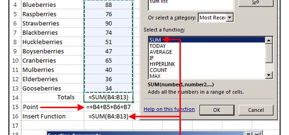
SUM, AVERAGE, COUNT: These are the building blocks of any data analysis.

The SUM function adds up a range of numbers, helping you quickly total expenses, scores, or any other numerical data. The AVERAGE function calculates the mean of a range of numbers, which is great for finding the typical value in your data set. The COUNT function counts the number of cells that contain numbers, which is useful for understanding how many entries you have.

For example, if you have a list of sales numbers in column A from A1 to A10:

• Use =SUM(A1:A10) to find the total sales.
• Use =AVERAGE(A1:A10) to find the average sales.
• Use =COUNT(A1:A10) to see how many sales entries are there.

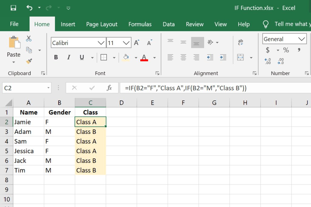
IF Statements: The IF function lets you create conditional statements in your spreadsheet. It works by evaluating a condition and returning one value if the condition is true and another value if it’s false. This is perfect for situations where you need to categorize data or make decisions based on specific criteria.

For instance, if you want to mark sales above $1000 as “Good” and below as “Needs Improvement”: Use =IF(A1>1000, “Good”, “Needs Improvement”).

2. Advanced Formulas

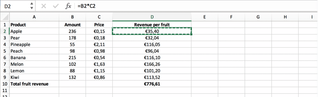
ARRAYFORMULA: This function can make your life easier by applying a formula to an entire range of cells at once, instead of entering it multiple times. It’s particularly handy for performing repetitive tasks across rows or columns.

For example, if you want to multiply each value in column A by 2 and place the results in column B: Use =ARRAYFORMULA(A1:A10*2) in cell B1.

VLOOKUP and HLOOKUP: These functions are your go-to tools for searching data across tables. VLOOKUP (Vertical Lookup) searches for a value in the first column of a range and returns a value in the same row from another column. HLOOKUP (Horizontal Lookup) does the same but searches across the top row.

For example, if you have a list of products in column A and their prices in column B, and you want to find the price of a product listed in D1: Use =VLOOKUP(D1, A1:B10, 2, FALSE) to get the price.

QUERY: The QUERY function allows you to perform complex data manipulations using SQL-like syntax. It’s powerful for sorting, filtering, and transforming your data.

For instance, if you want to select all rows where sales are greater than $1000: Use =QUERY(A1:B10, “SELECT * WHERE B > 1000”).

3. Data Validation

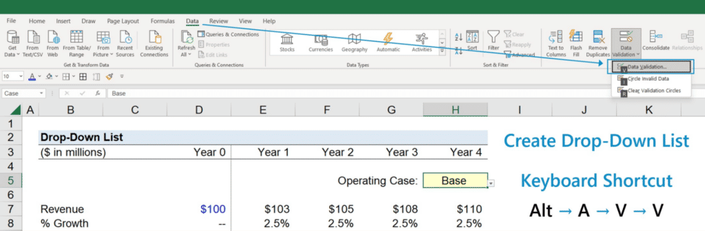
Dropdown Lists: Creating dropdown lists can help you standardize input values, making your data more consistent and easier to analyze. This is especially useful in shared sheets where multiple users enter data.

To create a dropdown list:

• Select the cells where you want the dropdown.
• Go to Data > Data validation.
• Choose “List of items” and enter your desired options separated by commas (e.g., “Yes, No, Maybe”).

Custom Data Validation Rules: Custom data validation ensures that the data entered into your sheets meets specific criteria. This can help prevent errors and maintain data quality.

For example, if you want to ensure that a column only contains numbers between 1 and 100:

• Select the cells.
• Go to Data > Data validation.
• Choose “Number” and set the criteria to “between” and enter 1 and 100.

4. Conditional Formatting

Color Coding Cells: Conditional formatting allows you to automatically apply color coding to your cells based on their content. This makes it easy to highlight important data trends at a glance. For instance, you can set it up so that cells with sales figures above a certain threshold are green, and those below are red.

To set up color coding:

• Select the range of cells you want to format.
• Go to Format > Conditional formatting.
• Set the conditions (e.g., greater than 1000) and choose the formatting style (e.g., green fill).

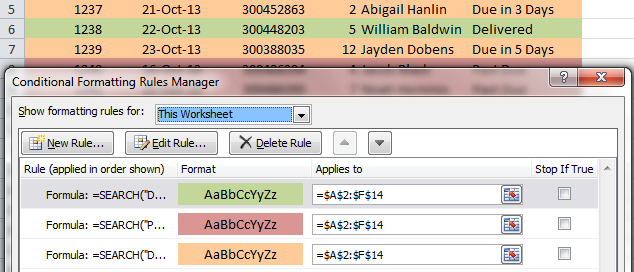
Custom Formatting Rules: You can create custom rules to apply more specific formatting based on multiple conditions. For example, you might want to highlight cells that are empty or contain errors.

To create custom rules:

• Select your range of cells.
• Go to Format > Conditional formatting.
• Click on “Add another rule” and set your custom conditions.

5. Pivot Tables

Creating Pivot Tables: Pivot tables are incredibly useful for summarizing large data sets. They allow you to quickly see totals, averages, counts, and other statistics by different categories without altering the original data.

To create a pivot table:

• Select your data range.
• Go to Data > Pivot table.
• Drag and drop fields into the Rows, Columns, Values, and Filters sections to organize your data.

Customizing Pivot Tables: Once your pivot table is created, you can customize it by adding filters, changing the data aggregation methods, and adjusting the layout to better suit your needs.

For example, to filter your pivot table to show only sales data for a specific month:

• Click on the filter drop-down in the pivot table.
• Select the desired month from the list.

6. Google Sheets Add-ons

Installing Add-ons: Google Sheets supports a variety of third-party add-ons that can extend its functionality. These add-ons can help with tasks like data cleaning, automation, and advanced analysis.

To install an add-on:

• Go to Extensions > Add-ons > Get add-ons.
• Browse the available add-ons and click “Install” on the ones you need.

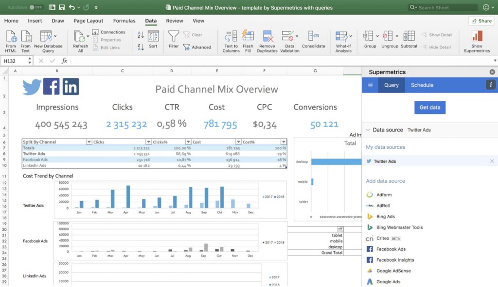
Popular Add-ons: Some add-ons can greatly enhance your Google Sheets experience. Here are a few popular ones:

• Supermetrics: Ideal for pulling data from marketing platforms like Google Analytics, Facebook Ads, and more.

• Power Tools: A suite of tools for data manipulation, including advanced find and replace, data cleaning, and more.
• Advanced Find and Replace: Helps you search for and replace data with more precision and options than the standard find and replace function.

10 Best Google Sheets Add-ons to Enhance Productivity

7. Collaboration Features

Real-time Collaboration: One of the best features of Google Sheets is the ability to collaborate with others in real time. Multiple users can work on the same sheet simultaneously, with changes appearing instantly. This is great for team projects, allowing everyone to contribute and see updates as they happen.

To start collaborating:

• Click on the “Share” button in the top right corner.
• Enter the email addresses of the people you want to share with.
• Set their permission level (view, comment, or edit) and click “Send.”

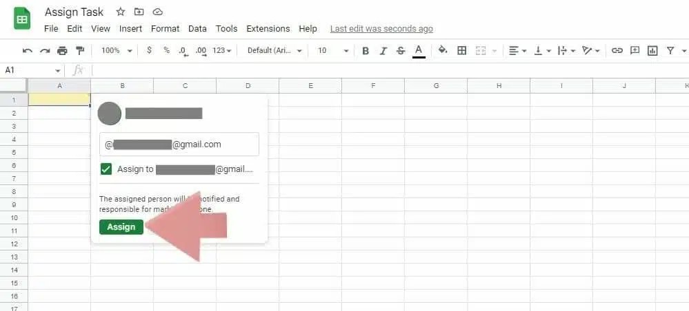
Commenting and Assigning Tasks: You can leave comments on specific cells to provide feedback or ask questions. Additionally, you can assign tasks to team members directly within the sheet.

To add a comment:

• Right-click on a cell and select “Comment.”
• Type your comment and click “Comment.”
• To assign a task, use the “+” symbol followed by the person’s email address (e.g., [email protected]) and then add your comment.

8. Data Import and Export

Import Data from Google Forms: Google Forms can automatically collect responses and send them to a Google Sheet. This is useful for surveys, quizzes, and feedback forms, allowing you to analyze responses in a structured format.

To link a Google Form to a Google Sheet:

• Create your form in Google Forms.
• Click on the “Responses” tab and then on the green Sheets icon.
• A new sheet will be created where all form responses will be collected.

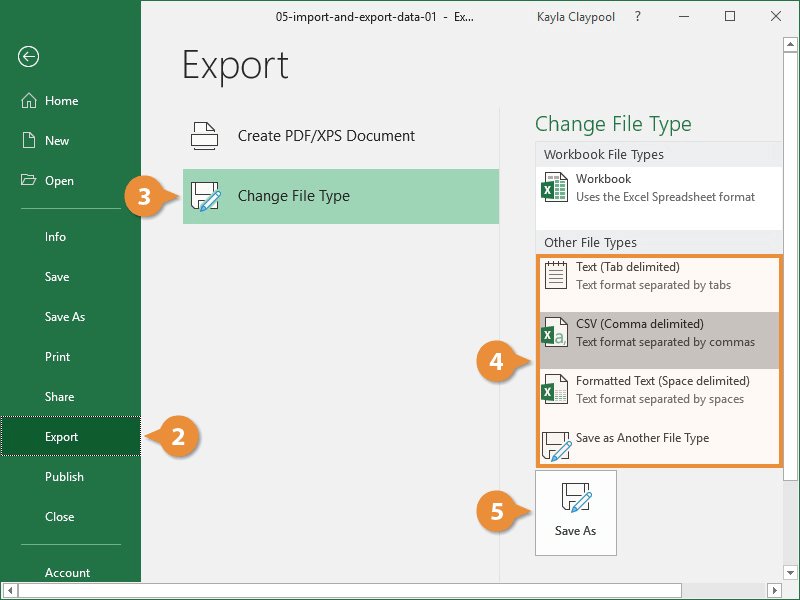
Export Data to Different Formats: Google Sheets allows you to export your data in various formats, such as CSV, Excel, and PDF. This makes it easy to share your data with others who might be using different software.

To export your data:

• Go to File > Download.
• Choose the format you need (e.g., Microsoft Excel, PDF, CSV).
• The file will be downloaded to your computer.

9. Automation with Google Apps Script

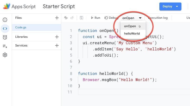
Google Apps Script is a powerful tool that allows you to automate tasks and extend the functionality of Google Sheets using JavaScript. With Apps Script, you can write custom functions, automate repetitive tasks, and integrate Google Sheets with other Google services.

To access Google Apps Script:

• Go to Extensions > Apps Script.
• A new window will open where you can write and run your scripts.

Simple Automation Examples: Here are a couple of simple examples of what you can do with Google Apps Script:

• Automate data entry: Create a script to automatically populate cells based on specific criteria.
• Send email notifications: Write a script that sends email alerts when certain conditions in your sheet are met.

10. Using Macros

Recording Macros: Macros in Google Sheets allow you to automate repetitive tasks without writing code. You can record a series of actions and then play them back with a single click, saving you time and effort.

To record a macro:

• Go to Extensions > Macros > Record macro.
• Perform the actions you want to automate.
• Click “Save” and give your macro a name.

Running and Editing Macros: Once you’ve recorded a macro, you can easily run it whenever you need. You can also edit the macro’s script to make adjustments or add more functionality.

To run a macro: Go to Extensions > Macros and select the macro you want to run.

To edit a macro:

• Go to Extensions > Macros > Manage macros.
• Click on the three dots next to the macro and select “Edit script.”

11. Data Analysis and Cleaning Tools

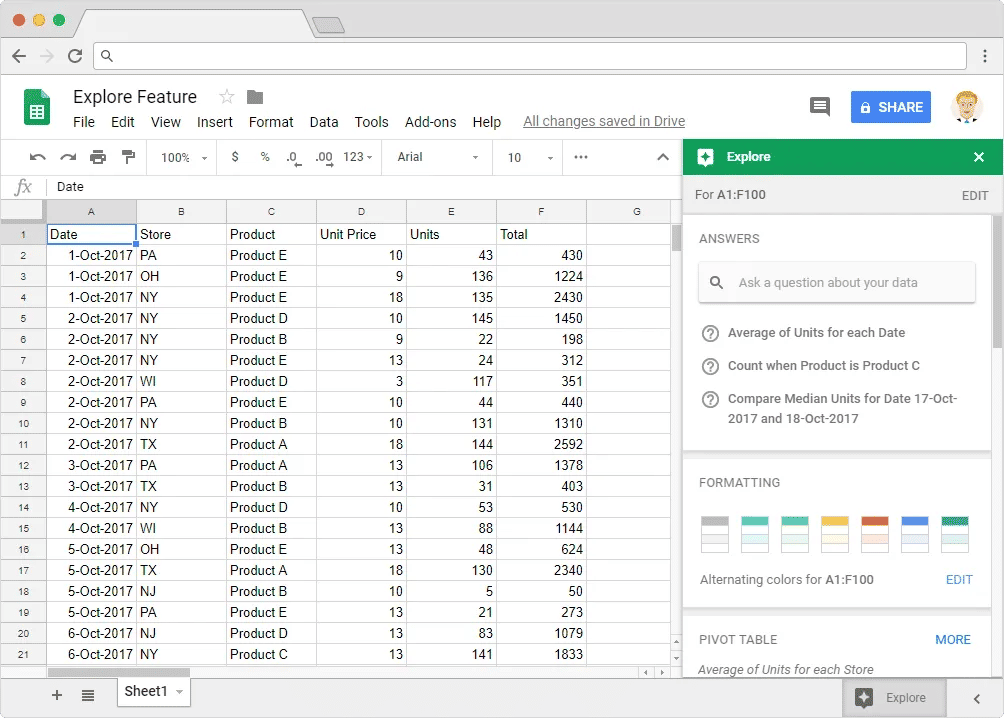
Explore Tool: The Explore tool in Google Sheets provides quick insights and visualizations based on your data. It can automatically generate charts, pivot tables, and statistical summaries, making it easier to understand and analyze your data.

To use the Explore tool:

• Select the data range you want to analyze.
• Click on the Explore icon (the star-shaped button at the bottom right) or go to Tools > Explore.
• The Explore panel will open on the right side, offering suggestions and insights.

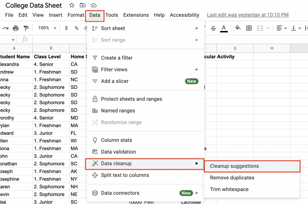
Data Cleaning: Google Sheets offers several features to help you clean and organize your data, ensuring accuracy and consistency. These tools can remove duplicates, split text into columns, and more.

To remove duplicates:

• Select the range of cells.
• Go to Data > Data cleanup > Remove duplicates.

To split text into columns:

• Select the column with the text you want to split.
• Go to Data > Split text to columns.
• Choose the delimiter (e.g., comma, space) to split the text.

12. Protecting and Sharing Sheets

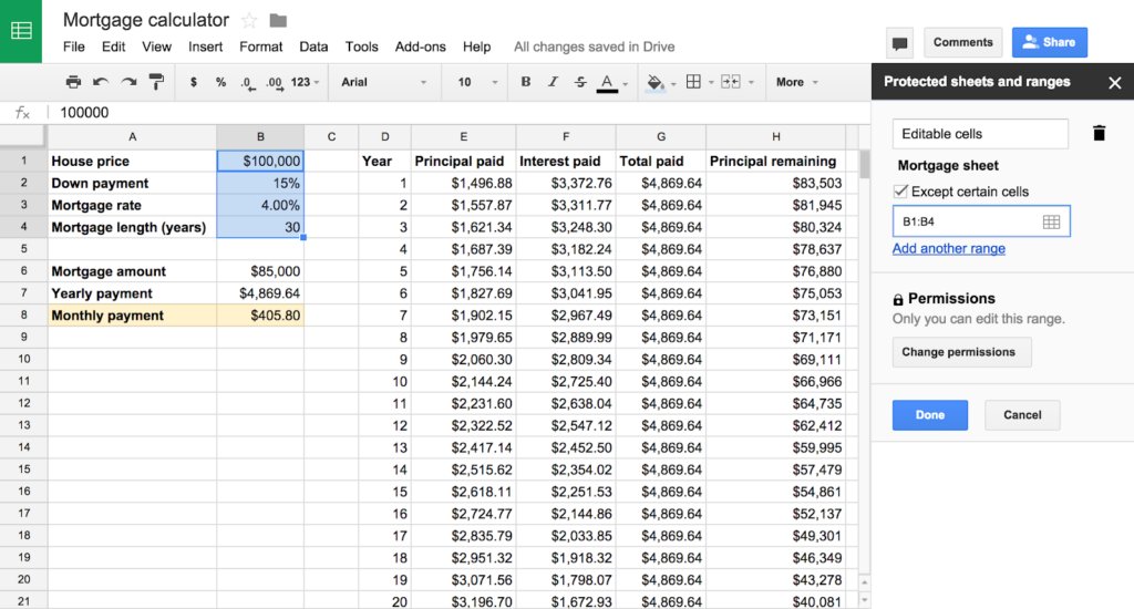
Protecting Sheets and Ranges: To prevent accidental edits or unauthorized changes, you can protect entire sheets or specific ranges. This is useful for keeping critical data intact while still allowing others to view or edit other parts of the sheet.

To protect a sheet or range:

1. Select the range or sheet you want to protect.
2. Go to Data > Protect sheets and ranges.
3. Set the permissions and click “Done.”

Sharing Options: Google Sheets offers flexible sharing options, allowing you to control who can view, comment, or edit your sheets. You can share with specific people via email or generate a shareable link with customized permissions.

To share a sheet:

1. Click on the “Share” button in the top right corner.
2. Enter the email addresses of the people you want to share with.
3. Set their permission level (view, comment, or edit) and click “Send.”

13. Keyboard Shortcuts

Essential Shortcuts: Keyboard shortcuts can save you a lot of time by allowing you to perform common actions quickly. Here are a few essential shortcuts to help you work faster in Google Sheets:

• Ctrl + C (Cmd + C on Mac): Copy
• Ctrl + V (Cmd + V on Mac): Paste
• Ctrl + Z (Cmd + Z on Mac): Undo
• Ctrl + Y (Cmd + Y on Mac): Redo
• Ctrl + F (Cmd + F on Mac): Find
• Ctrl + Shift + V (Cmd + Shift + V on Mac): Paste values only

Custom Shortcuts: You can also create custom shortcuts for actions you frequently use. While Google Sheets doesn’t have a built-in feature for creating custom shortcuts, you can use browser extensions like AutoHotkey (for Windows) or create custom shortcuts on your Mac.

14. Integrating with Other Google Services

Google Data Studio: Google Data Studio is a powerful tool for creating interactive reports and dashboards from your Google Sheets data. This integration allows you to visualize and share your data in a more engaging way.

To connect Google Sheets with Data Studio:

• Open Google Data Studio.
• Click on “Create” and choose “Data source.”
• Select “Google Sheets” and choose the sheet you want to connect.

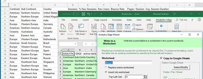
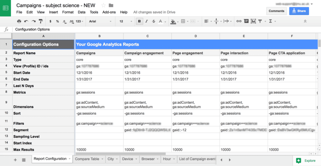
Google Analytics Integration: If you’re using Google Analytics, you can import your analytics data directly into Google Sheets. This allows you to create custom reports and dashboards using your website data.

To import Google Analytics data:

1. Install the Google Analytics add-on from the Google Workspace Marketplace.
2. Open your sheet, go to Extensions > Add-ons > Get add-ons, and search for Google Analytics.
3. After installing, go to Extensions > Google Analytics > Create new report and follow the prompts.

15. Mobile App Usage

Google Sheets Mobile App: The Google Sheets mobile app allows you to work on your spreadsheets while on the go. It offers most of the functionality available on the desktop version, so you can view, edit, and share your sheets from anywhere.

To use the mobile app:

• Download and install the Google Sheets app from the App Store (iOS) or Google Play Store (Android).
• Sign in with your Google account.
• Open your sheets and start working.

Mobile-Specific Features: The mobile app also includes features specifically designed for mobile use, such as offline mode and voice input. Offline mode allows you to work on your sheets without an internet connection, and your changes will sync when you’re back online. Voice input lets you enter data by speaking, which can be handy when you’re on the move.

To enable offline mode:

1. Open the Google Sheets app.
2. Tap on the three dots next to the sheet you want to make available offline.
3. Toggle the “Available offline” switch.

16. Version History and Recovery

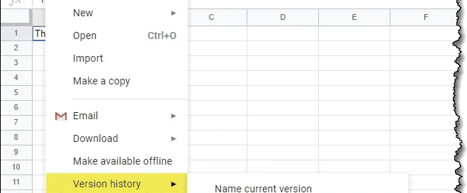
Viewing Version History: Google Sheets keeps a detailed version history of your document, allowing you to track changes and revert to previous versions if needed. This is incredibly useful for collaborative projects where multiple people are making edits.

To view version history:

• Go to File > Version history > See version history.
• A panel will open on the right, showing a list of versions with timestamps and editor names.
• Click on any version to see what changes were made and, if needed, restore that version.

Restoring Previous Versions: If you need to revert to an earlier version of your sheet, you can do so easily. This can help recover data that might have been accidentally deleted or changed.

To restore a previous version:

• Follow the steps to view version history.
• Find the version you want to revert to and click on it.
• Click “Restore this version” at the top of the panel.

17. Using Templates

Accessing Google Sheets Templates: Google Sheets offers a wide range of templates for various needs, from budgets and invoices to project management and calendars. Using templates can save you time by providing a pre-made structure that you can customize to fit your needs.

To access templates:

• Go to Google Sheets homepage.
• Click on “Template gallery” at the top right.
• Browse through the available templates and click on the one you want to use.

Custom Templates: If you frequently create similar types of spreadsheets, you can create your own custom templates. This ensures consistency and saves time in setting up new sheets.

To create a custom template:

• Design your sheet with the necessary structure and formatting.
• Save it with a clear, descriptive name.
• When you need to use it, open the template, make a copy (File > Make a copy),and start working with the copy.

18. Latest Features and Updates

Connected Sheets: Connected Sheets is a feature that integrates Google Sheets with BigQuery, Google’s powerful data warehouse solution. This allows you to handle and analyze large datasets directly within Google Sheets without having to write complex SQL queries.

To use Connected Sheets:

• You need to have access to BigQuery.
• Open a Google Sheet and go to Data > Data connectors > Connect to BigQuery.
• Follow the prompts to link your BigQuery data.

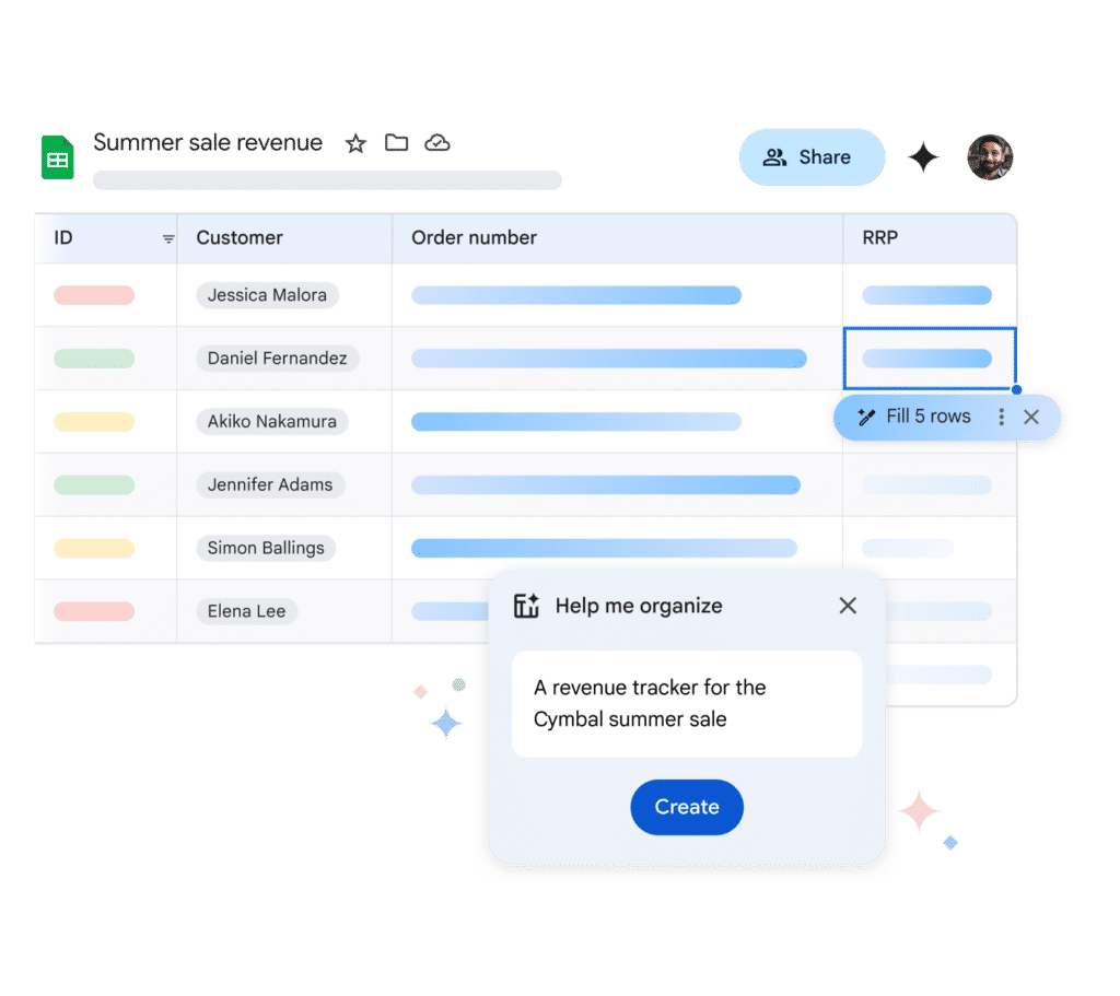
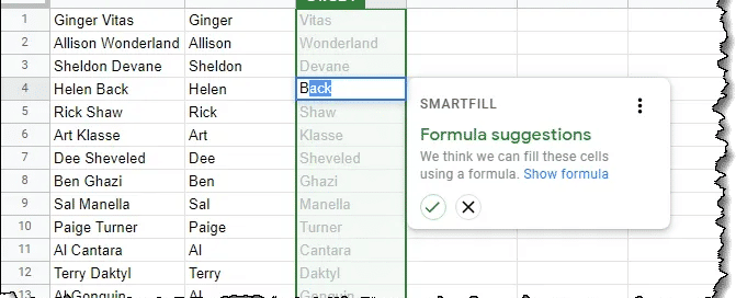
Smart Fill:Smart Fill is an AI-driven feature that helps you with data entry by predicting and suggesting what you’re typing based on patterns in your data. It’s similar to autocomplete and can save a lot of time, especially with repetitive tasks.

To use Smart Fill:

• Start typing in a cell, and if Smart Fill detects a pattern, it will suggest a fill.
• Press Enter to accept the suggestion or continue typing to ignore it.

Conclusion

Google Sheets might seem simple at first glance, but it’s packed with features that can really make your life easier. Whether you’re crunching numbers, managing projects, or collaborating with a team, there’s a tool or trick in Google Sheets to help you do it better.

With these 18 tips, I’ve covered a lot of ground, from basic functions and advanced formulas to automation and integration. Each functionality is designed to save you time and boost your productivity.

Don’t be afraid to play around with these features and see how they can fit into your workflow. The more you experiment, the more you’ll find new ways to make Google Sheets work for you.